{{ title }}
{{ category }}
Role: Research Assistant · Team: 1 · Timeline: 7 months
OVERVIEW
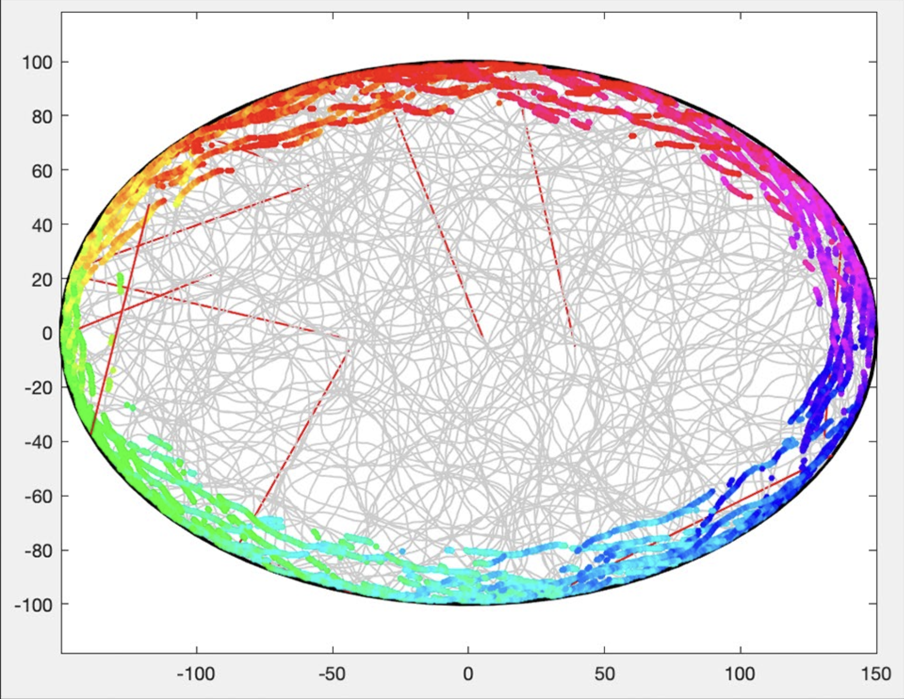
The Hasselmo Laboratory works on simulating neural behavior responsible for navigation. The grey lines on figures shown represent a rodent’s trajectory through an environment and the colored dots represent the locations in which certain neurons fire. The laboratory's goal is to experiment with different mathematical models for neural firing, and see which can most accurately correspond to real rodent brain activity. It focuses primarily on egocentric boundary cells, which are neurons that fire when an animal reaches a boundary, and grid cells, which are neurons that fire when an animal enters any location in an environment that falls on part of a predetermined hexagonal grid.
MY ROLE
- Creating a new, more efficient and straightforward ray tracing script that allows the user to easily create custom environments for the simulation.
- Creating and simulating real and imaginary trajectories for forward scanning, working one on one with the professor to implement the oscillatory interference model to predict when neurons will fire.
- Debugging and speeding up pre-existing MATLAB scripts achieving over 50% speed improvement.
Tools & Tech
Custom Ray Tracing Script
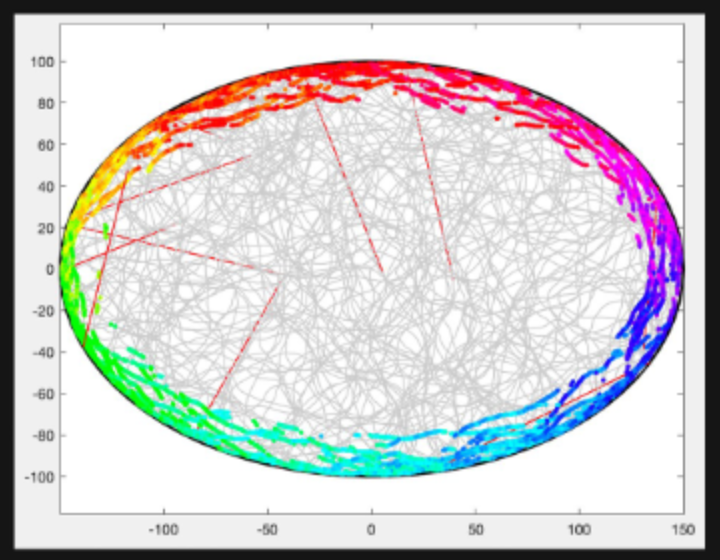
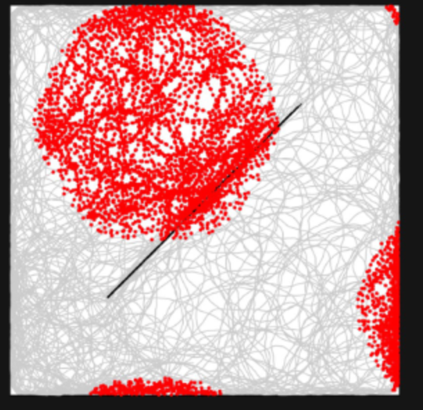
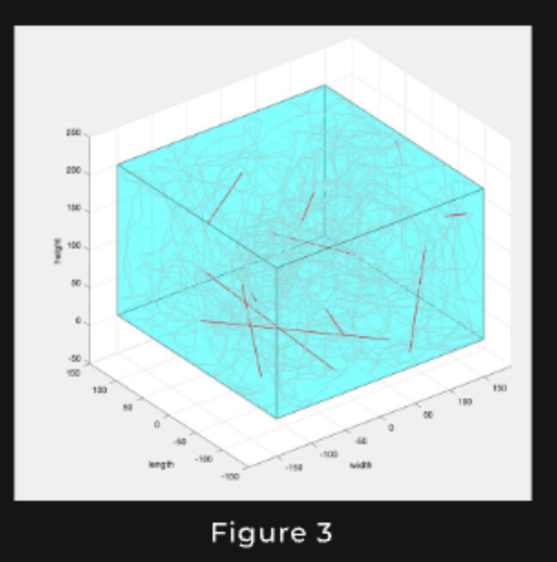
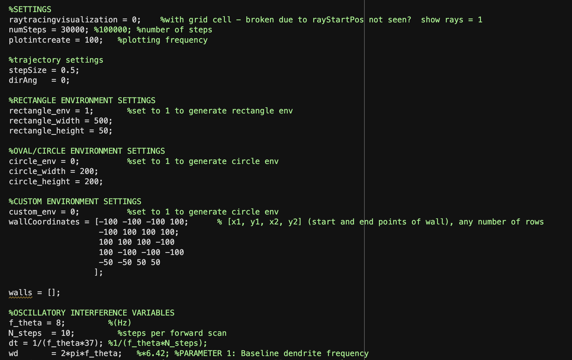
The previous rodent trajectory script that the laboratory had ran slowly, had bugs, could not support barricades, and was difficult to use. Therefore, I was tasked with creating a better ray tracing script. I created a randomly generated trajectory and then implemented ray tracing to sense and avoid barriers. While before the environment had to be changed manually in the code, my new script let the user pick from a rectangular, circular (Fig. 1) or a custom environment at the top of the script using a few variables. It can also be easily configured to have barriers (Fig. 2). The ray tracing was necessary to have the same algorithm work in any environment, and to implement logic for boundary cell firing, which I added after the script was complete. I also implemented a grid cell firing model which is based on the sum of oscillations from three head directions that vary with direction and speed, as well as the brain’s baseline theta rhythm. I also later implemented a 3D version of the ray tracing script for the same purpose (Fig. 3).
Neural Forward Scanning Script
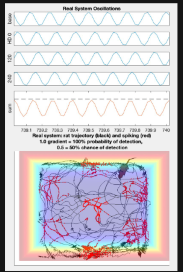
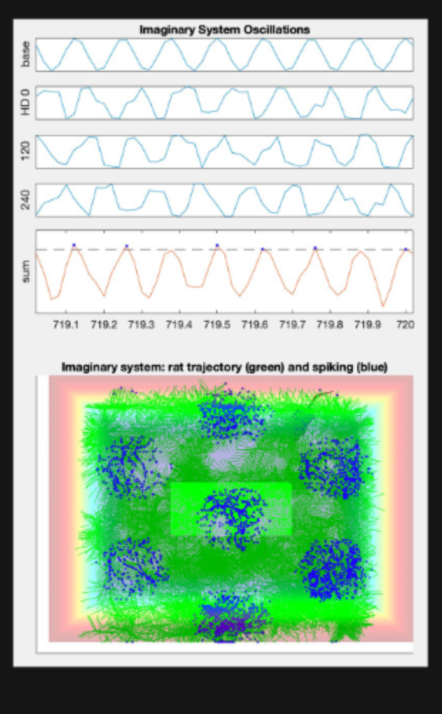
I created a script that simulated both the real and imaginary trajectories of a rodent (this time without ray tracing and instead using a gaussian distribution to simulate behavior at boundaries). The imaginary trajectory followed that of the real trajectory, but with additional “forward scans” that form the resulting green pattern. I then created a visualization of the sum of oscillations from the baseline theta rhythm and three head directions for both the imaginary and real trajectories. When the sum reached a threshold, the grid cells fired, resulting in the hexagonal pattern seen, which was expectedly more defined for the imaginary trajectory.
WITH GRID CELL FIRINGS
WITH GRID CELL FIRINGS