{{ title }}
{{ category }}
Role: C Code & ML Training · Team: 3 · Timeline: 2 weeks
Overview
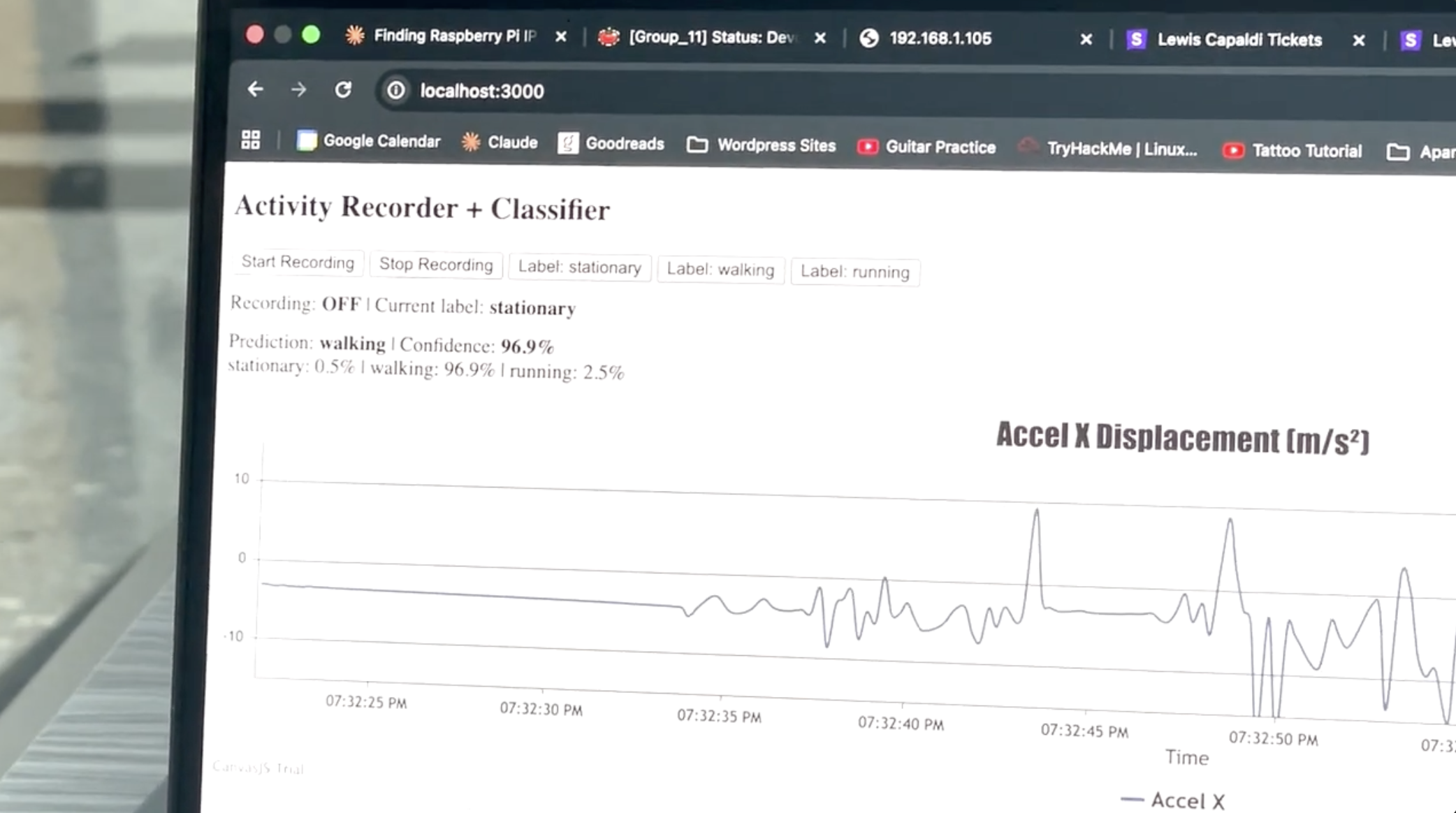
We combined I2C sensor interfacing with wifi connectivity and Machine Learning applications. We used an ESP32 to read data from an accelerometer unit via I2C and stream that data over a UDP connection to a socket running in nodejs application. That application recorded that data in a CSV format along with the appropriate data label as well as displayed the data live via an html server. The recorded data was used to train an ML model that was then used to classify new incoming data and display its prediction on the same html server.
My Role
- Wired and integrated the initial accelerometer and lidar setup.
- Fine tuned the machine learning settings for the best classification results.
Tools & Tech
Overview
We implemented live sensor localization using an ESP32 with a LiDAR (LIDAR-Lite v4) and an accelerometer (ADXL343) on a shared breadboard. The goal was to stream sensor data over USB serial to a Node.js server, compute displacement from both sensors, and visualize everything in a browser dashboard so you can compare LiDAR vs. accelerometer displacement for accuracy testing.
To get it working we: (1) ran the ESP32 firmware (ESP-IDF) that polls LiDAR and accelerometer over I2C and logs tagged lines at 115200 baud; (2) built a Node.js server that opens the serial port, parses those log lines with regexes, double-integrates acceleration into displacement and uses the first LiDAR reading as a baseline to report LiDAR displacement; (3) served a single-page HTML dashboard over HTTP and pushed parsed data in real time via Socket.IO to CanvasJS charts—four rows: per-axis acceleration, accelerometer displacement, LiDAR displacement, and a comparison chart of both displacements.
Hardware
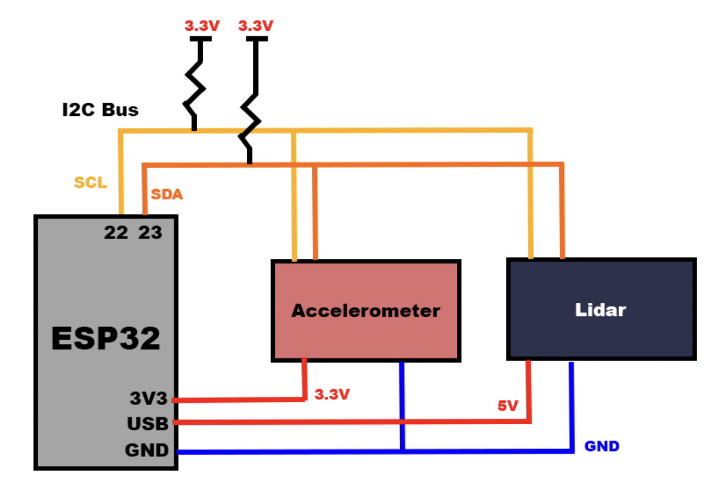
LIDAR AND ACCELEROMETER CONNECTED TO ESP32 VIA THE SAME I2C BUS ON GPIOS 22 AND 23.
Software
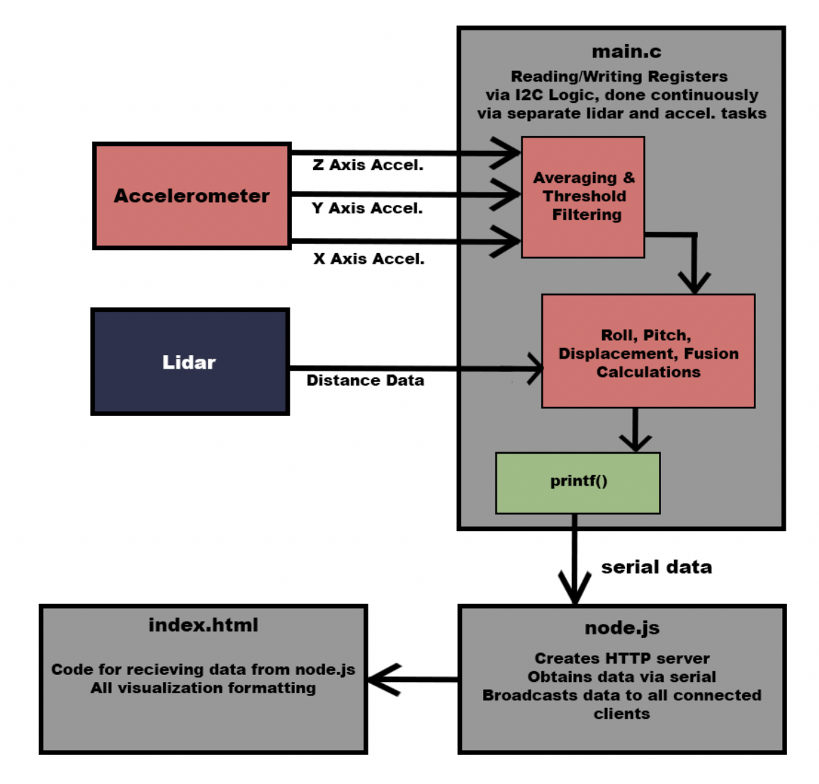
SEPARATE LIDAR AND ACCELEROMETER TASKS IN MAIN.C, FILTERING AND FUSION ON DEVICE, THEN SERIAL TO NODE AND OUT TO THE BROWSER.
Outcome
We got real-time LiDAR and accelerometer data streaming to the browser with displacement computed on the server and displayed in four rows of charts. The comparison chart (chart on row 4 of server) lets you see which accelerometer axis best matches LiDAR displacement when you move the breadboard along the LiDAR’s line of sight.
Dataflow
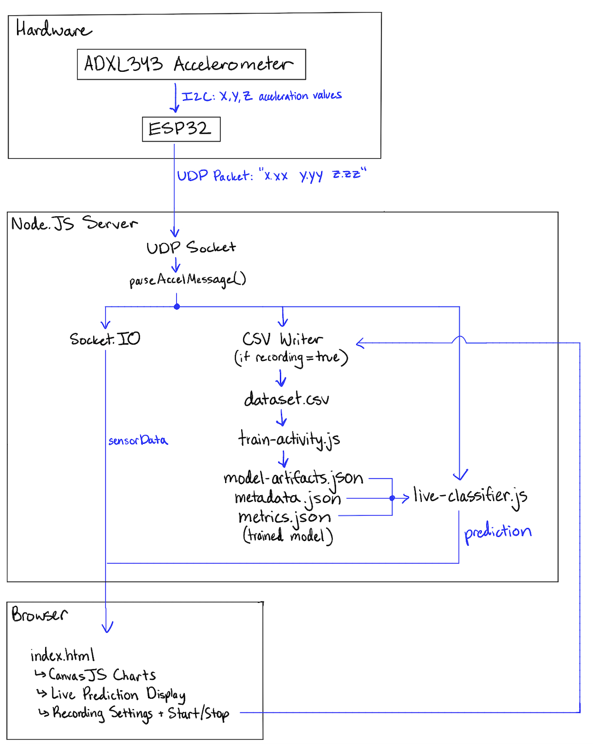
ACCELEROMETER TO ESP32 OVER I²C, ESP32 TO NODE OVER UDP, NODE TO THE BROWSER OVER SOCKET.IO — WITH THE CSV AND THE TRAINED MODEL BRANCHING OFF THE SAME STREAM.
Accelerometer Readings and Web Dashboard
We used the accelerometer setup from the first part of this project to read the X, Y, and Z acceleration values and send them to the ESP32 over I2C. These values were then sent over Wifi UDP to Node, with the ESP32 configured as a client that pushed the data to the IP of the Raspberry Pi on the same network. It used sendto() to push the data string of acceleration values continuously. Since the ESP32 doesn’t wait for a response, unlike TCP, this allows for faster data transfer. Node is then used to host a local server, to which it passes the accelerometer data using SocketIO. The browser then displays real-time graphs of the accelerations using CanvasJS and HTML. For ease of data collection for training, our dashboard also features start and stop recording buttons as well as a label that assigns a mode (stationary, walking, or running), which initiates the recording of the data to a CSV file with the corresponding label.
Machine Learning
This data was then used to train our model by running the training script, which takes 20 data points from the CSV at a time, computes their mean and standard deviation, and adjusts the values accordingly so that the data can be interpreted based on how far off from the “average” value it is, which makes training faster and more reliable. It also divides the data into training (for learning), validation (to monitor for overfitting), and testing (measuring accuracy) buckets. To improve the accuracy of our model, we collected stationary, walking, and running data from all members of our group. After initial training, our web dashboard displays a real-time prediction for the data being fed into it after every 20 samples.
Results
Final confusion matrix
This indicates 100% accuracy on the training data for stationary and walking modes, but only 66% accuracy for walking. This is likely due to the fact that our walking pace was too slow and also too similar to our running pace, so there was not a high level of differentiation in the dataset. This could have also been improved by collecting more data for walking, however, since we collected over 2000 datapoints, for Roger’s sanity, we decided to call it a day.
Failure Case Analysis
In order to get to this point, we first tried training the model on a dataset only 400 lines long, which resulted in a confusion matrix of:
FIRST ATTEMPT, TRAINED ON A 400-LINE DATASET.
This, along with having a confidence level of near 50% while making predictions, did not make for a very good model. Therefore, we analyzed our data and noticed that when switching between modes, we sometimes mixed running data with walking data, walking data with stationary data, and vice versa. To fix this, we implemented a simple button interface in our browser so that we could stop and start the recording at any time, and preemtively select the label for the data. Furthermore, we collected many more samples from our accelerometer (positioned at the ankle) by recording for longer periods of time and sending the data to the CSV more frequently than before. We also chose to halve our training window from 20 to 40, and increase the epochs, so that the model would have more instances to train from and train on them longer. The final confusion matrix was the result of these efforts.
Back to All Projects